A Structural equation modeling
A.1 What does SEM accomplish?
You can think of sem as reg (or OLS) with much more flexilibity (but also comes with depth and complexities), where gsem is the generalized version. It is good for handling unobservables, correlations, and coefficient constraints. As an example for unobservables, with given certain assumptions, an investigator might use multiple academic performance metrics to infer intelligence — the latent variable. Vanilla bivariate SEM will result in exactly the same results as bivariate OLS, but beyond bivariate specifications, SEM’s flexibility on how it treats covariances and autocorrelations for multiple variables makes it a useful modeling technique. On top of this, we can give the model constraints if we (happen to) know the (true) value of a coefficient or just to give it a quick test. Without a doubt, it requires strong assumptions especially because of its flexibilities, but gives a bit of leeway for OLS’ limitations.
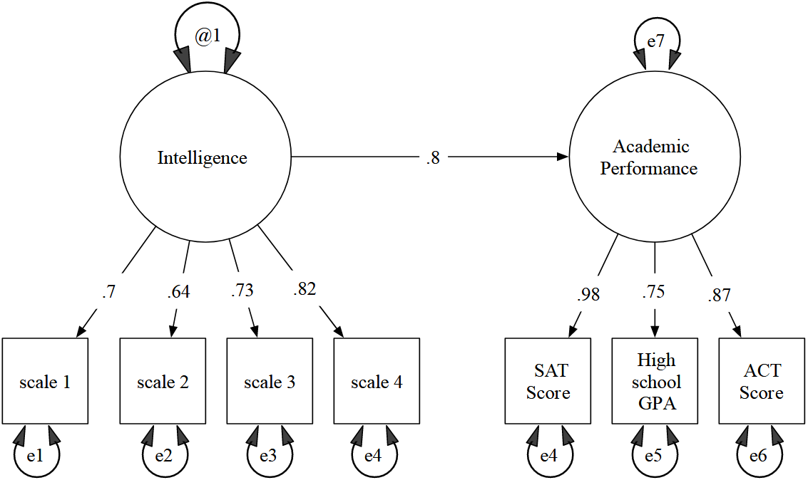
In the above diagram, intelligence and academic performance are latent variables, while the boxes are observed variables.
Notes
This statistical technique was used by Boyan Zheng for Louise’s research. The rest of the section will show a reduced version of their work for demonstration purposes. Also, this method should not be confused with structural models in econometrics and economics.
Also note that in Stata’s documentation for SEM, the lingo for “path coefficient” means beta coefficient.
.do file that combines all the chunks of Stata commands is provided at the end.
A.2 What was their goal?
Their goal was to see what kind of relationship different variables had on husbands and wives. The following are the reduced version of their research questions.
- What kind of effects does wife + husband depression have on husband + wife social life?
- What kind of intra and inter relations can we draw from them given that they live in the same household?
In order to set this up, we have to set up a CESD scoring system, reshape the NSHAP data so the CESD/social activity are into separate variables for husbands and wives. As a side note, there are few non-heterosexual observations in the data.
If you would like to learn more about the scoring system, check out NSHAP’s own publication “Measuring Social Isolation among Older Adults Using Multiple Indicators from the NSHAP Study” by Cornwell and Waite in the journals of gerontonology series b of psychological sciences, volume 64B, supplment 1 (November 2009). It is freely available online and hardcopies are available freely in the NORC office! You can see that this tutorial’s method is somewhat similar if you take a quick look at the table in page i41.
A.3 The set up
A.3.1 CESD scoring
First, let’s create a score variable for all of the depression variables. Essentially, the scoring is set up as an ordinal variable for each of the depression variables, then all of the depression ordinal variables combined. There are definitely concerns with this, but will be (partially) addressed later. Let’s take a look at one of the CESD variables first, namely noteat.
. tab noteat

   cesd: did not feel like |
                    eating |      Freq.     Percent        Cum.
---------------------------+-----------------------------------
rarely or none of the time |      3,467       72.68       72.68
          some of the time |        741       15.53       88.22
              occasionally |        392        8.22       96.44
          most of the time |        170        3.56      100.00
---------------------------+-----------------------------------
                     Total |      4,770      100.00
Looking at the above output, this is what the scoring would translate to:
1: rarely or none of the time
2: some of the time
3: occasionally
4: most of the time
And similar story applies to rest of the CESD variables, fltdep, ftleff, nosleep, etc. Note that washapy and enjlife are in reverse order, so when we come to the part where we combine the CESD variables to create a score, make sure to change the two variables’ order to match the ordinality with rest of the CESD variables with the commands gen r_enjlife = 5 - enjlife and gen r_washapy = 5 - washapy. Now, let’s combine them and see what the result looks like.
. gen cesd_score = r_washapy + r_enjlife + noteat + fltdep + flteff + nosleep + waslonly + unfriend + fltsad + dislikd + notgetgo

. tab cesd_score

 cesd_score |      Freq.     Percent        Cum.
------------+-----------------------------------
         11 |        599       12.71       12.71
         12 |        518       11.00       23.71
         13 |        495       10.51       34.22
         14 |        453        9.62       43.83
         15 |        370        7.85       51.69
         16 |        334        7.09       58.78
         17 |        270        5.73       64.51
         18 |        261        5.54       70.05
         19 |        212        4.50       74.55
...
Since there were 11 CESD variables, 11 being the minimum makes sense.
A.3.2 Concern with CESD scoring system
The unavoidable concern for validity is combining the CESD variables into one simple measure like above. Not only that, it is a combination of ordinal variables, which became a continuous variable. Furthermore, it does not help that each of the CESD variables’ correlation values do not seem very promising. Here is a truncated output:
. corr noteat fltdep flteff nosleep washapy waslonly unfriend enjlife fltsad dislikd notgetgo

             |   noteat   fltdep   flteff  nosleep  washapy waslonly unfriend  enjlife   fltsad  dislikd notgetgo
-------------+---------------------------------------------------------------------------------------------------
      noteat |   1.0000
      fltdep |   0.3005   1.0000
      flteff |   0.3391   0.4391   1.0000
     nosleep |   0.2321   0.2973   0.2894   1.0000
...
However, correlation is only a measurement of standard deviations and covariances. Correlation’s weakness lies in the fact that it does not account for shared covariances between the numerous variables. This is where Cronbach’s alpha comes in.
A.3.3 Cronbach’s alpha (\(\tau\)-equivalent reliability)
Cronbach’s alpha is a measurement of reliability over multiple variables — though the word “consistency” might be better to understand it. Basically, alpha shows that answers were consistently picked for the questions. Although SEM is better compatible with Raykov’s composite reliability (AKA congeneric reliability), it is not (yet) available in Stata, even though it is a more modern replacement for alpha. Further, alpha does not perform very well with missing data and checking \(\tau\)-equivalency adds a bit of stringency (which tends to be overlooked in the literature).
A researcher should go through the due diligence for the mentioned concerns, but for demonstration purposes, we will briefly go over what the process looks like. Let’s see how Cronbach’s alpha looks for the CESD variables.
. drop if partner_id == ""
. alpha noteat fltdep flteff nosleep washapy waslonly unfriend enjlife fltsad dislikd notgetgo

Test scale = mean(unstandardized items)
Reversed items: washapy enjlife

Average interitem covariance:     .1741151
Number of items in the scale:           11
Scale reliability coefficient:      0.8041
0.8041 is a solid number to work with. Although there is no general rule of thumb for alpha, rule of thumb for congeneric reliability is that we want 0.7 or higher.
A.3.4 Reshaping data by husband/wife partners
In order to continue with the SEM modeling, we have to make sure that our data is compatible to our research question for Stata to understand in variables. This requires the command reshape. Here is a visual explanation, given in Stata’s documentation.
   long
+------------+                  wide
| i  j  stub |                 +----------------+
|------------|                 | i  stub1 stub2 |
| 1  1   4.1 |     reshape     |----------------|
| 1  2   4.5 |   <--------->   | 1    4.1   4.5 |
| 2  1   3.3 |                 | 2    3.3   3.0 |
| 2  2   3.0 |                 +----------------+
+------------+
In our case, i is hh_id or household ID, and j is gender. We are trying to convert our data into the wide format, so we will have new variables for husbands and wives. However, Stata requires that j has unique values within each i. This means that in the data, gender variable contains only two values, 1 and 2. Since there are only two values, this means that there should be only two observations per household in order for them to be unique observations per household. This unique-value-per-household rule also goes same for other variables; this means that we cannot use the given weight_adj variable anymore (though we can still keep cluster and stratum). Let’s only keep the variables of interest for now. You can also choose to keep cluster and stratum.
keep hh_id gender cesd_score waslonlyFor demonstration purposes, we will use partner_id variable, which is the su_id of their partner respondent. The only catch of this demonstration is that even though some NSHAP respondents are partnered, they are not necessarily in the NSHAP data. Let’s start with dropping observations with missing partner_id with the command keep if partner_id != "" or drop if partner_id == "".
To fit with the said research questions and for demonstration purposes, let’s focus on hetero partners. Summing up the gender with the two partners in the same household, and checking whether that sum is 3 makes sure that one partner is female and other is male (2 and 1).
. sort hh_id
. by hh_id: egen sum_gender = sum(gender)
. keep if sum_gender == 3
Now, we are ready run the reshape command. Let’s see how it looks and rename the variables for readability.
. reshape wide cesd_score social, i(hh_id) j(gender)
. list in 1/5

     +-----------------------------------------------------------------------------+
     |   hh_id                social1   cesd_s~1                social2   cesd_s~2 |
     |-----------------------------------------------------------------------------|
  1. | 1000001             every week         12   several times a year         16 |
  2. | 1000005             every week         15             every week         14 |
  3. | 1000009   several times a week         17             every week         25 |
  4. | 1000013             every week         11             every week         14 |
  5. | 1000021                  never         19   several times a year         18 |
     +-----------------------------------------------------------------------------+

. ren social1 social_husband
. ren social2 social_wife
. ren cesd_score1 cesd_husband
. ren cesd_score2 cesd_wife
During the reshape process, Stata automatically assigns the two gender values to the variable names. So in the above output, cesd_s~1 means CESD score for husband, while cesd_s~2 means CESD score for wife. Now, we are ready to execute some SEM commands!
A.4 Use SEM in Stata
Going back to the research question mentioned previously, we are trying to predict how CESD explains social life. In other words, our \(y\) variable is social, while our \(x\) variables is the CESD score. Since we are investigating a discrete variable, we use gsem instead of sem (which become essentially the same if working with continuous variable). Here is how to set up the structural equation with a truncated output. Note that the command works fine without the covariance option.
. gsem (i.social_husband -> cesd_wife) (i.social_husband -> cesd_husband) (i.social_wife -> cesd_wife) (i.social_wife -> cesd_husband), cov(e.cesd_husband*e.cesd_wife)

Generalized structural equation model           Number of obs     =      1,075
...
Log likelihood = -6319.4902

-------------------------------------------------------------------------------------------------
                                |      Coef.   Std. Err.      z    P>|z|     [95% Conf. Interval]
--------------------------------+----------------------------------------------------------------
cesd_wife                       |
                 social_husband |
         less than once a year  |  -.1796659   2.029517    -0.09   0.929    -4.157445    3.798114
    about once or twice a year  |  -1.521126   1.724117    -0.88   0.378    -4.900333    1.858081
          several times a year  |  -3.255614    1.60672    -2.03   0.043    -6.404728   -.1065003
            about once a month  |  -3.838579   1.599506    -2.40   0.016    -6.973553   -.7036041
                    every week  |  -3.396186   1.593948    -2.13   0.033    -6.520267   -.2721047
          several times a week  |   -3.47962   1.617088    -2.15   0.031    -6.649054   -.3101854
                                |
                    social_wife |
         less than once a year  |   3.006314    2.25652     1.33   0.183    -1.416384    7.429011
    about once or twice a year  |   .3544712   1.687279     0.21   0.834    -2.952534    3.661476
          several times a year  |  -.1305966   1.588978    -0.08   0.934    -3.244936    2.983742
            about once a month  |  -.6342675   1.574404    -0.40   0.687    -3.720043    2.451508
                    every week  |  -1.401933   1.566622    -0.89   0.371    -4.472455    1.668589
          several times a week  |  -1.928945   1.592559    -1.21   0.226    -5.050303    1.192413
                                |
                          _cons |   20.85038   1.987248    10.49   0.000     16.95545    24.74532
--------------------------------+----------------------------------------------------------------
cesd_husband                    |
                 social_husband |
         less than once a year  |    2.61445     1.8641     1.40   0.161    -1.039119    6.268019
...
--------------------------------+----------------------------------------------------------------
                var(e.cesd_wife)|   25.02529   1.081345                      22.99316    27.23702
             var(e.cesd_husband)|   19.91174   .8648453                      18.28682    21.68105
--------------------------------+----------------------------------------------------------------
 cov(e.cesd_wife,e.cesd_husband)|   3.951548   .7003826     5.64   0.000     2.578823    5.324272
-------------------------------------------------------------------------------------------------
Interpreting the coefficients is similar to mlogit; we can interpret the signs, but not the magnitude.
As a side note, when Stata is calculating the maximum likelihood, it should neither be backed up nor its functional form be convex. If Stata notifies (backed up) or (not concave) for the maximum likelihood iterations, then restrategizing the model may be necessary, or the direction of the prediction from the independent variables to the dependent variables may need restructuring.
A.4.1 Simple SEM comparison to OLS
Try comparing the outputs from reg cesd_wife social_husband and sem (social_husband -> cesd_wife) commands.
A.5 Estimating the first two moments
In Stata, there are few neat features that comes with SEM that lets you estimate the first and second moments (though conditions are slightly different for GSEM). The first moment means the mean, and the second moment means the variance. More specifically for SEM however, you can
- Estimate the moments
- Not estimate the moments
- Constrain a coefficient to a fixed value
- Constrain two or more moment coefficients to be equal
From the previous gsem output, the results for the covariance are reporting that there is slight covariance on CESD between the partners and it is statistically significant. Notice that rest of the results are the same as before, except for the maximum likelihood. For sem, similar story applies to noxconditional option, which is used by default when constraints are applied to the mean, variance, and/or covariance.
For the other three options, see help sem and gsem path notation in the Stata documentation.
A.6 Comparing coefficients
After running a model, changing the magnitudes between different coefficients may help understand the model’s specification a bit better, relating one coefficient to another. In other words, you might want to know the difference between x2 and x3 on their effects on the \(y\) variable. You can use lincom or nlcom for (non-)linear comparisons, where non-linear comparison allows for non-linear expressions such as division.
To give an example scenario from the above gsem specification, an investigator might be curious on the effects of husband’s social activity compared to wife’s social activity, maybe to see which has a bigger effect on wife’s CESD score.
. lincom [cesd_wife]2.social_wife - [cesd_wife]2.social_husband
...
------------------------------------------------------------------------------
             |      Coef.   Std. Err.      z    P>|z|     [95% Conf. Interval]
-------------+----------------------------------------------------------------
         (1) |  -1.875598   2.596621    -0.72   0.470    -6.964882    3.213687
------------------------------------------------------------------------------
In the command, 2. means the second ordinal value, in which case would be “some of the time” value. And because this is a comparison, the formulation is subtraction, whereas if we were to see the effects of both of their social activity to wife’s CESD score, then we would use addition. If need be, the relative-risk ratio option can be used with , rr. Looking at the results above, it seems that wife’s social activity would contribute more towards wife’s CESD scoring compared to husband’s social activity; this sounds reasonable, but the statistical significance shows that the model performs poorly on accuracy, most likely due to the sample size. This can also be alleviated if there were fewer answer choices, so there are more samples per answer.
For other functional forms and methods such as logit, see help lincom in the Stata documentation.
A.7 Marginal effects and graphing
GSEM with discrete \(y\) variable specification cannot directly interpret the magnitudes of coefficients, which is similar to logit and its derivatives. This means that an extra step is necessary for investigating marginal effects. What we need to do is select a point in the domain and see what the marginal effect of that point is. Stata automatically chooses the middle point for you. Then, let’s make a graph of the margins.
. margins social_wife
. marginsplot, xdimension(social_wife) horizontal ytitle("Wife socializing")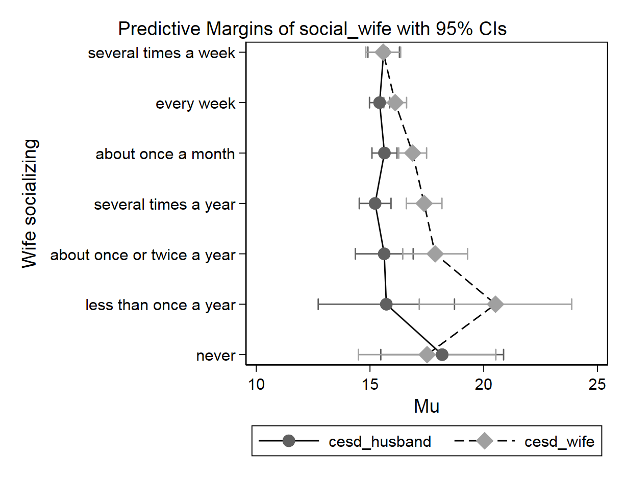
Looking at the above graph, it is apparent that there may be sample size issues for certain answers, especially for “never” answer. Beyond that, this shows that wife’s different levels of social activity does not have much effect on husband’s CESD score. In the x-axis, “Mu” stands for “marginal units” for CESD score.
A.8 .do file
use "P:\5707\ARC\W3\Release as of 12-06-18\nshap-3.0b3\w3\nshap_w3_core.dta"

gen r_enjlife = 5 - enjlife
gen r_washapy = 5 - washapy
gen cesd_score = r_washapy + r_enjlife + noteat + fltdep + flteff + nosleep + waslonly + unfriend + fltsad + dislikd + notgetgo

keep if partner_id != ""

sort hh_id
by hh_id: egen sum_gender = sum(gender)
keep if sum_gender == 3

keep hh_id gender cesd_score social

reshape wide cesd_score social, i(hh_id) j(gender)
list in 1/5

ren social1 social_husband
ren social2 social_wife
ren cesd_score1 cesd_husband
ren cesd_score2 cesd_wife

gsem (i.social_husband -> cesd_wife) (i.social_husband -> cesd_husband) (i.social_wife -> cesd_wife) (i.social_wife -> cesd_husband), cov(e.cesd_husband*e.cesd_wife)

lincom [cesd_wife]2.social_husband - [cesd_wife]2.social_wife

margins social_wife
marginsplot, xdimension(social_wife) horizontal ytitle("Wife socializing")