Part 4 OLS
4.1 What is OLS?
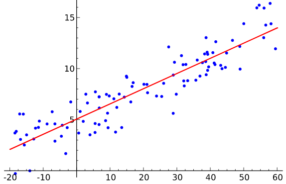
OLS stands for ordinary least squares; it fits a line through data points like the picture above. A basic OLS is a good preliminary step for statistical analysis. It quickly draws an approximate picture how much impact a variable has on another variable (magnitude) and whether they have a positive or negative relationship. However, it should be noted that plain OLS estimations should not be used as a final step of a research.
4.2 Simple example — the math step by step
As an example, let’s just look at 2 variables for now — \(x\) and \(y\). The formula for a regression is \(y_i = \beta _0 + \beta _1 x _i + \varepsilon _i\). In order to find out the impact of \(x\) on \(y\), we have to find the value of \(\beta _1\) using OLS. The formula for that is \(\beta _1 = \frac{var(x)}{cov(x,y)}\). Another way of writing this is \(\beta _1 = \frac{(x - \bar{x})^2}{(x - \bar{x})(y - \bar{y})}\). Watch this super simple, 8-minute video on how to get the \(\hat\beta _1\) by hand: https://www.youtube.com/watch?v=JvS2triCgOY
4.3 In Stata
Since this is a survey with clusters, strata, and weights, let’s make sure we tell Stata that this is a survey data. Check if it is already set up using the command svyset.
. svyset

      pweight: weight_adj
          VCE: linearized
  Single unit: missing
     Strata 1: stratum
         SU 1: cluster
        FPC 1: <zero>
If the output does not look like this, then run the command svyset cluster [pw = weight_adj], str(stratum). This makes sure that our regression accounts for clusters, strata, and weights.
Now, on to OLS: when Stata performs an OLS, it also carries out many other functions simultaneously. For sake of example, let the \(y\) variable be hearn (household earning) and \(x\) be age. Let’s take a look at the output of the survey regression and talk about few commonly discussed values. Note that svy: is a prefix command that tells Stata account for clusters, strata, and weights.
. svy: reg hearn age
(running regress on estimation sample)

Survey: Linear regression

Number of strata   =        50                  Number of obs     =      2,423
Number of PSUs     =       100                  Population size   = 2,467.7556
                                                Design df         =         50
                                                F(   1,     50)   =      29.78
                                                Prob > F          =     0.0000
                                                R-squared         =     0.0226

------------------------------------------------------------------------------
             |             Linearized
       hearn |      Coef.   Std. Err.      t    P>|t|     [95% Conf. Interval]
-------------+----------------------------------------------------------------
         age |  -1955.745   358.3929    -5.46   0.000    -2675.598   -1235.891
       _cons |   202385.9   27774.05     7.29   0.000     146600.1    258171.7
------------------------------------------------------------------------------
Starting with the equation, our \(y\) variable is hearn, while our \(x\) variable is age. So our OLS formula would be \(hearn = \beta _0 + \beta _1 age + \varepsilon\).
From the OLS formula, the \(\beta _1\) is -1955.745. This shows that for every 1 unit (year) increase in age, household earning decreases by an average 1955.745 units (dollars). (Remember the ages of the survey sample!)
Though not commonly discussed, for sake of interpretation, _cons is our \(\beta _0\). This means that if age was 0, our mean hearn would be 202385.9.
Since the 95% confidence interval for age does not include 0 for age, it is statistically significant within 95% confidence interval. Similarly, P>|t| also tells us that since it is smaller than 0.05, it is statistically significant at the 5% significance level.
R-squared looks extremely low, but that is expected since we only used age variable as our regressor. As you add more \(x\) variables, the specification will explain more of the variation in the \(y\) variable, meaning R-squared will increase. The value 0.0226 tells us that age explains about 2.26% of the variance in hearn.
4.4 Handling discrete variables
If the \(y\) variable is a discrete variable, then Stata cannot perform an OLS estimation. However, it can perform OLS if \(x\) variables are discrete. In order to estimate with discrete \(x\) variables, the prefix i. has to be attached to the \(x\) variable. An example Stata command would be reg y i.x1 i.x2 x3 x4 i.x5.