Part 5 Logit
5.1 Goal of logit
The goal of logit is to calculate the odds of landing heads on a coin flip or a binary variable. For example, what is the probability that an NSHAP respondent saying “yes” to a question? Let’s use the variable college as the dependent variable; it asks “did you attend college or university?” and it is coded as 1 for yes, 0 for no.
5.2 What about probit?
This is a commonly asked question. Although the functional forms are drastically different for probit and logit, they surprisingly come to a very similar conclusion when drawing inference from the same data. Logit is a bit more popular than probit because logit can easily calculate the odds ratio (risk). For this exercise, we will just focus on logit and how we have to be careful about coefficients.
. svy: logit college i.ethgrp age hearn
(running logit on estimation sample)

Survey: Logistic regression

Number of strata   =        50                  Number of obs     =      2,413
Number of PSUs     =       100                  Population size   = 2,460.8854
                                                Design df         =         50
                                                F(   5,     46)   =      16.78
                                                Prob > F          =     0.0000

--------------------------------------------------------------------------------------
                     |             Linearized
             college |      Coef.   Std. Err.      t    P>|t|     [95% Conf. Interval]
---------------------+----------------------------------------------------------------
              ethgrp |
              black  |   -.431153     .21434    -2.01   0.050    -.8616676   -.0006385
hispanic, non-black  |   -.636324   .2598162    -2.45   0.018     -1.15818   -.1144678
              other  |  -.0458698    .438495    -0.10   0.917     -.926613    .8348733
                     |
                 age |  -.0175393   .0066775    -2.63   0.011    -.0309515    -.004127
               hearn |   .0000198   4.82e-06     4.11   0.000     .0000101    .0000295
               _cons |   .7080575   .6725172     1.05   0.297     -.642733    2.058848
--------------------------------------------------------------------------------------
Note: 0 failures and 6 successes completely determined.
5.3 How to read the coefficients for discrete \(x\) variables
Notice that under ethgrp variable, the white cateogory is missing. The way discrete \(x\) variables are calculated are by setting a base value. In this case, the base value is white. Although we cannot yet interpret the values yet, let’s take a look at the sign for black. What this negative sign here means is that black tend to have lower probability of attending college compared to the base value, white. For OLS, you can read the coefficient value directly. Assuming that the OLS output gave -0.431153 for sake of an example, it would mean that black would have 43.1153% lower probability than white on attending college.
5.4 How do we determine the marginal values?
Getting the marginal value is equivalent of taking the derivative. However, since logit functional form is not linear, we have to take the derivative given certain \(x\) values. This means that we can only get marginal value after telling Stata where to take the derivative. So, let’s just say white, 70 years old, with household income 150,000. What would be the probability of attending college given these \(x\) values? We have to use the margins command.
. margins, atmeans at(ethgrp=1 age=70 hearn=150000)

Adjusted predictions                            Number of obs     =      2,413
Model VCE    : Linearized

Expression   : Pr(college), predict()
at           : ethgrp          =           1
               age             =          70
               hearn           =      150000

------------------------------------------------------------------------------
             |            Delta-method
             |     Margin   Std. Err.      t    P>|t|     [95% Conf. Interval]
-------------+----------------------------------------------------------------
       _cons |   .9207264    .035118    26.22   0.000     .8501898    .9912629
------------------------------------------------------------------------------
The result above shows that given that a person is white, 70 years old, with a household income is 150,000, they have ~92.07% probability that they attended college. The value of P>|t| = 0.000 shows that it is statistically significant.
5.5 Graphing logit
. qui svy: logistic college age hearn i.gender i.rested
. predict y_hat
. tw line y_hat hearn, sort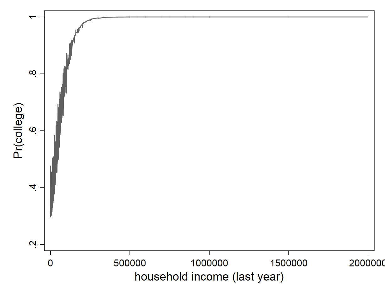
First, the description of a standard representation of a logit regression – actually, it is the inverse of logit, which is the logistic regression. The above shows the probability of attending college from 20% to 100% on the y-axis. On the x-axis, it shows household income. This is the case if the \(x\) variable is continuous. (The graph does not imply causality.)
In order to graph a discrete variable, we have to follow slightly different commands. Use margins and marginsplot instead. (Try it!)
//svy: logistic college age hearn i.gender i.rested //(no need to run this command twice)
. margins rested
. marginsplot
For both cases, you can plot multiple \(x\) variables by adding more \(x\) variables to the commands. Scales might become a problem, however.