Part 2 Chi-squared test

2.1 What is chi-squared?

\(\chi ^2\) is for a preliminary step of a statistical investigation, helping to determine whether samples in two categorical variables are observed by luck or not. It can test for independence of two categorical variables among other functions. Note that Fisher’s and Barnard’s exact tests are better, but computationally heavier – more on this later.

Explanation — independence

It compares expected number of sampled vs. actual observations. We will take a look at two different stories. First story will be to see whether gender and ethgrp (ethnic group) are independent or not, and the second story will be to see whether the two categorical variables par_nerve (“how often does your spouse/partner get on your nerves?”) and spdemand2 (“how often does spouse/partner make too many demands?”).

2.2 The first story — tabulate and \(\chi ^2\) on `gender` and `ethgrp`

Let’s start with the command tab ethgrp gender, chi2 which gives this output:

. tab ethgrp gender, chi2

     race/ethnicity |
          recode (4 | gender of respondent
        categories) |      male     female |     Total
--------------------+----------------------+----------
              white |     1,104      1,299 |     2,403 
              black |       217        300 |       517 
hispanic, non-black |       174        193 |       367 
              other |        39         39 |        78 
--------------------+----------------------+----------
              Total |     1,534      1,831 |     3,365 

          Pearson chi2(3) =   3.9497   Pr = 0.267

In our world, we think that race/ethnicity and gender are independent (ethnicity does not depend on your gender and vice versa). Even if we know they are, let’s pretend we don’t know for sake of an example (and because certain samples does not guarantee the right results, usually questionable sampling methods). In order to conduct a preliminary analysis on the independence hypothesis or the culture hypothesis for further research, we need to perform the \(\chi ^2\) test. For exact test, use the command tab ethgrp gender, exact.

2.2.1 The rule of thumb

The important number here is Pr = 0.267, which determines whether you reject the null hypothesis that the two variables are independent from each other or not. In this case, we fail to reject the null hypothesis at the 5% (for example) significance level because 0.267 is higher than 0.05. In short, the two variables are likely to be independent. If you know the math or already did it by hand, you can use the Stata command display chiprob(df,x) or the shortform di chiprob(df,x).

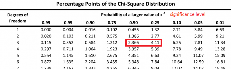
Just to cross-check, Pearson chi2(3) = 3.9497 tells us that the degrees of freedom is 3, and \(\chi ^2\) value is 3.9497. Looking at the table above, 3.9497 is between 2.366 and 4.11. This tells us a significance level somewhere between 0.5 and 0.25, which is way higher than the standard 0.1, 0.05, or 0.01. Therefore, we fail to reject the null.

2.2.2 Exact or \(\chi ^2\) test?

You should always use exact test if computationally possible. It definitely depends on the hardware specs, but with 2019 consumer-grade technology (i3/i5/i7 or Ryzen CPUs), exact test should be able to handle sample size in the 100,000s within a minute if not few seconds. Since exact and \(\chi ^2\) tests are just preliminary steps of a statistical analysis, it is most likely not worth the hours or days of computation, so if sample size is close to or higher than million, or if it takes more than a minute, use \(\chi ^2\) test.

2.3 The second story — tabulate and \(\chi ^2\) on `par_nerve` and `spdemand2`.

Reviewing the questions, “how often does your spouse/partner get on your nerves?” and “how often does spouse/partner make too many demands?” are seemingly dependent on each other, as well as correlated. The difference between the first story and this second story is that the categories of the second story has an order. To clarify, “often” is a higher (discrete) value than “some of the time” and so forth.

. tab par_nerve spdemand2, chi2

       how often does | how often does spouse/partner make too many
  partner get on your |                  demands?
              nerves? |     never  hardly ev  some of t      often |     Total
----------------------+--------------------------------------------+----------
                never |       117         61         20         13 |       211 
hardly ever or rarely |       269        364        139         40 |       812 
     some of the time |       155        345        281         98 |       879 
                often |        14         24         32         41 |       111 
----------------------+--------------------------------------------+----------
                Total |       555        794        472        192 |     2,013 

          Pearson chi2(9) = 300.3252   Pr = 0.000

2.3.1 Validity check

Are the categories within the variables mutually exclusive? More concretely, is “some of the time” exclusive to “hardly ever or rarely” for both variables? The answer is unlikely. Person A’s definition of “hardly ever or rarely” could be twice a month, but it could be twice a week for person B, which may be person A’s “some of the time” instead. For this reason, survey design is important and the NSHAP team has to pay due diligence on probing questions, adding supplemental details along the questions, or reformulate the answers entirely.