A Response rate prediction
A.1 The goal
As of writing this tutorial, we have up to NSHAP wave 3. Using these W2 and W3 databases, we will:
Find what proportion/probability of respondents from wave 2 completes the NSHAP questionnaire or not and
See how well this probability carries over to wave 3 to determine if it is usable for wave 4
The main strength of this prediction technique is that the conditional probabilities can be easily transferred over to different databases (such as the NIH’s) because of its simple approach. Simply put, the question is “given certain characteristics, what is the probability that this person will complete the NSHAP survey?”
A.1.1 Notes
This statistical technique was used by Jin-Kyu Choi/Jack Coghlan for Colm’s research in SAS. The rest of the section will show a reduced version of their work. R script that combines all the code chunks is provided at the end.
A.2 The set up with W2
First, we have to find the conditional probabilities for W2. The wave 2 data is P:\5707\5707B\Administrative\Research Assistant Essentials\NSHAP Stata Training Materials\R tutorial winter 2019\nshap_w3_core.xlsx (W3 data is the same as before, but this will be covered later). Let’s import that first.
#w2 <- read_excel("P:/5707/5707B/Administrative/Research Assistant Essentials/NSHAP Stata Training Materials/R tutorial winter 2019/nshap_w2_core.xlsx")

w2 %>%
    select(su_id, hh_id, fi_id, path, surveytype, category2, ageelig, partner, version2) %>%
    head()
## # A tibble: 6 x 9
## su_id hh_id fi_id path surveytype category2 ageelig partner version2
## <chr> <chr> <chr> <chr> <chr> <chr> <chr> <chr> <chr>
## 1 10000~ 10000~ 1805~ 6 W1 NIR partner in~ 1 0 partner
## 2 10000~ 10000~ 4359~ 6 partner partner in~ 1 1 partner
## 3 10000~ 10000~ 6605~ 4 W1 R partner in~ 1 0 partner
## 4 10000~ 10000~ 6605~ 4 partner partner in~ 1 1 partner
## 5 10000~ 10000~ 3958~ 4 W1 R not applic~ 1 0 no part~
## 6 10000~ 10000~ 4153~ 3 W1 R partner in~ 1 0 partnerThere are whopping 889 variables! For demonstration purposes, let’s reduce it down to gender and race for personal characteristics. As for defining what constitutes as “completing the questionnaire” in this case, let’s simply define that if we have invalid data for 150 questions or more, it will count as an incomplete; this means that since there are 889 variables, they should have 150 or fewer “not applicable” data points per row. Let’s create a variable to count the number of “not applicable” (not “NA” in R, but as string “not applicable” from the Excel file) for each row first. After that, we can create a binary variable that either meets or does not meet threshold.
w2 <- w2 %>%
    mutate_all(as.character)

w2_completes <- w2 %>%
    mutate(count_na = rowSums(. == "not applicable")) %>%
# . or the dot works with %>% or the "pipe" to call w2 into the function;
# essentially, it is equivalent to rowSums(w2 == "not applicable").
    mutate(completed = (count_na < 150))

# Let's see how many completes and incompletes there are
w2_completes %>%
    group_by(completed) %>%
    summarise(n = n())
## # A tibble: 3 x 2
## completed n
## <lgl> <int>
## 1 FALSE 1706
## 2 TRUE 1659
## 3 NA 12Note: converting the data as string or “character” is not best practice, but easier to work with for demonstration purposes. This solves couple of things. 1) it keeps leading zeroes in ID variables (though that should already be the case when importing the data), and 2) it makes upcoming string comparison code easier to work.
Now, let’s reduce the number of variables and remove w2 and w2_completes dataframes for efficiency.
w2_comp_selected <- w2_completes %>%
    select(gender, race, completed)

#rm(w2, w2_completes)

head(w2_comp_selected)
## # A tibble: 6 x 3
## gender race completed
## <chr> <chr> <lgl>
## 1 female white/caucasian TRUE
## 2 male white/caucasian TRUE
## 3 male white/caucasian TRUE
## 4 female white/caucasian TRUE
## 5 female white/caucasian FALSE
## 6 male white/caucasian FALSEWe are all set to go for wave 2! Using this dataframe, you can now generate conditional probabilities of completing the survey, where the conditions are given gender and race variables.
A.3 Generating conditional probabilities for W2
So, which cohorts are likely to complete our questionnaire? Let’s first divide the number of people that completed the survey by the total number of people to get the probability per gender per race cohorts.
w2_probs <- w2_comp_selected %>%
    group_by(gender, race) %>%
    summarise(n = n(), completes = sum(completed, na.rm = T)) %>%
    mutate(p2 = completes / n)

w2_probs %>%
    arrange(desc(p2)) %>%
    head()
## # A tibble: 6 x 5
## # Groups: gender [2]
## gender race n completes p2
## <chr> <chr> <int> <int> <dbl>
## 1 female american indian or alaskan native 10 6 0.6
## 2 female don't know 5 3 0.6
## 3 female asian or pacific islander 21 12 0.571
## 4 male black/african american 217 113 0.521
## 5 female refused 2 1 0.5
## 6 female white/caucasian 1402 696 0.496Just to see what the data looks like, it seems that highest rates of response rates are from females in general, though there are concerns such as missing data.
A.4 W3
Now, all we have to do is replicate the previous code for setting up the data and generating probabilities. We can combine all the W2 code into one through continuous piping. Although it becomes unreadable since it is a giant block of text, since it is nearly identical code to the W2 code, there is no need to worry about readability.
w3 <- read_excel("P:/5707/5707B/Administrative/Research Assistant Essentials/NSHAP Stata Training Materials/R tutorial winter 2019/nshap_w3_core.xlsx")

w3 <- w3 %>%
    mutate_all(as.character)

w3_probs <- w3 %>%
    mutate(count_na = rowSums(. == "not applicable")) %>%
    mutate(completed = (count_na < 150)) %>%
    group_by(completed) %>%
    select(gender, race, completed) %>%
    group_by(gender, race) %>%
    summarise(n = n(), completes = sum(completed, na.rm = T)) %>%
    mutate(p3 = completes / n)

w3_probs %>%
    arrange(desc(p3)) %>%
    head()
## # A tibble: 6 x 5
## # Groups: gender [2]
## gender race n completes p3
## <chr> <chr> <int> <int> <dbl>
## 1 female don't know 4 4 1
## 2 male american indian or alaskan native 19 11 0.579
## 3 male other 175 89 0.509
## 4 male white/caucasian 1566 753 0.481
## 5 male black/african american 321 137 0.427
## 6 female white/caucasian 1890 798 0.422Interestingly enough, there seems to be higher rates of responses from males in this wave. Note that there are concerns such as missing data as mentioned before. Either way, now that the W2 and W3 datasets have very similar variables, we can now merge them!
A.5 Merging W2 and W3
If you are familiar with SQL or its variants, then this should look familiar. The tidyverse library comes with several different methods for dataframe joining, such as left_join, inner_join, etc.
df_w2_w3 <- w2_probs %>%
    full_join(w3_probs, by = c("gender", "race"))

df_w2_w3 %>%
    arrange(desc(p2 + p3)) %>%
    head()
## # A tibble: 6 x 8
## # Groups: gender [2]
## gender race n.x completes.x p2 n.y completes.y p3
## <chr> <chr> <int> <int> <dbl> <int> <int> <dbl>
## 1 female don't know 5 3 0.6 4 4 1
## 2 male american indian o~ 15 6 0.4 19 11 0.579
## 3 male white/caucasian 1198 589 0.492 1566 753 0.481
## 4 female asian or pacific ~ 21 12 0.571 61 24 0.393
## 5 female american indian o~ 10 6 0.6 17 6 0.353
## 6 male other 84 37 0.440 175 89 0.509In order to compare the probabilities between the waves, we can subtract their differences to see how they compare:
df_w2_w3 <- df_w2_w3 %>%
    mutate(diff = p2 - p3)

df_w2_w3 %>%
    select(-completes.x, -completes.y, -p2, -p3) %>%
    arrange(desc(abs(diff))) %>% # absolute value
    head()
## # A tibble: 6 x 5
## # Groups: gender [2]
## gender race n.x n.y diff
## <chr> <chr> <int> <int> <dbl>
## 1 female don't know 5 4 -0.4
## 2 female american indian or alaskan native 10 17 0.247
## 3 female black/african american 300 470 0.185
## 4 male american indian or alaskan native 15 19 -0.179
## 5 female asian or pacific islander 21 61 0.178
## 6 male black/african american 217 321 0.0939Looking at the bigger sample size cohorts, it seems that the difference between the two waves are from 7 to 19 percentage points. Given that the sample sizes are 100 or more in each waves, median difference seems to be hovering somewhere around 8 percentage points.
A.6 Graphing
Now, in order to visualize the differences between the two waves, we can use the graphing techniques we learned from the previous section. Let’s visualize how different they are across race and gender.
race_diff <- df_w2_w3 %>%
    filter(race != "don't know" &
           race != "refused" &
           race != "not applicable") %>%
    ggplot() +
    geom_bar(aes(y = abs(diff),
                   x = race),
             stat = "identity") +
    facet_wrap(~gender, ncol = 1) +
    dark_theme_bw() +
    scale_y_continuous(limits = c(0, 0.5)) +
    coord_flip() +
    ggtitle("Differences in response rates between wave 2 and 3") +
    ylab("Absolute value of the differences")

ggsave(filename = "race_vs_diff.png",
       plot = race_diff,
       width = 12.8,
       height = 7.2,
       dpi = 150)

knitr::include_graphics("race_vs_diff.png")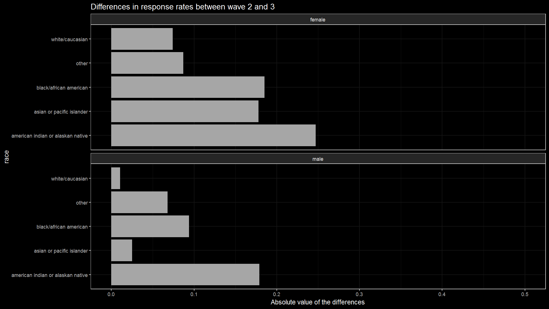
It seems that white/caucasian and male alongside asian or pacfic islander and male values are the most consistent between the two waves just by looking at this demonstration. This does not mean that they have the highest response rates, but rather it will (probably) be easier to predict whether they will respond or not, though this also depends on sample size. However, this simple conditional probability model can be expanded further by predicting weekly (and moving averages or smoothed means), adding more characteristics, diving the data by sample types, etc.
A.7 R script
rm(list=ls())

library(tidyverse)
library(readxl)

w2 <- read_excel("P:/5707/5707B/Administrative/Research Assistant Essentials/NSHAP Stata Training Materials/R tutorial winter 2019/nshap_w2_core.xlsx")

# wait a few seconds for it to load the data...

w3 <- read_excel("P:/5707/5707B/Administrative/Research Assistant Essentials/NSHAP Stata Training Materials/R tutorial winter 2019/nshap_w3_core.xlsx")


# W2

w2 <- w2 %>%
    mutate_all(as.character)

w2_completes <- w2 %>%
    mutate(count_na = rowSums(. == "not applicable")) %>%
    mutate(completed = (count_na < 150))

w2_completes %>%
    group_by(completed) %>%
    summarise(n = n())

w2_comp_selected <- w2_completes %>%
    select(gender, age, race, completed)

w2_probs <- w2_comp_selected %>%
    group_by(gender, race) %>%
    summarise(n = n(), completes = sum(completed, na.rm = T)) %>%
    mutate(p2 = completes / n)

#rm(w2, w2_completes)

w2_comp_selected %>%
    group_by(gender, age, race, completed) %>%
    summarise(n = n(), p = sum(completed))


# W3

w3 <- w3 %>%
    mutate_all(as.character)

w3_probs <- w3 %>%
    mutate(count_na = rowSums(. == "not applicable")) %>%
    mutate(completed = (count_na < 150)) %>%
    group_by(completed) %>%
    select(gender, race, completed) %>%
    group_by(gender, race) %>%
    summarise(n = n(), completes = sum(completed, na.rm = T)) %>%
    mutate(p3 = completes / n)

rm(w3)


# Merge W2 and W3

df_w2_w3 <- w2_probs %>%
    full_join(w3_probs, by = c("gender", "race"))

df_w2_w3 <- df_w2_w3 %>%
    mutate(diff = p2 - p3)

race_diff <- df_w2_w3 %>%
    filter(race != "don't know" & race != "refused" & race != "not applicable") %>%
    ggplot() +
    geom_bar(aes(y = abs(diff),
                   x = race),
             stat = "identity") +
    facet_wrap(~gender, ncol = 1) +
    dark_theme_bw() +
    scale_y_continuous(limits = c(0, 0.5)) +
    coord_flip() +
    ggtitle("Differences in response rates between wave 2 and 3") +
    ylab("Absolute value of the differences")

ggsave(filename = "race_vs_diff.png",
       plot = race_diff,
       width = 12.8,
       height = 7.2,
       dpi = 150)

knitr::include_graphics("race_vs_diff.png")