Part 3 Plotting, using `ggplot2`

3.1 Introduction

R has some serious capabilities for plotting. Note that the package is named ggplot2 while function or command is ggplot().

The ggplot2 system of plotting is quite modular. First, we initiate a graph with ggplot(), then you can add in different modules of a graph (for example, bar graph, text labels, colors, legend, title, etc.) with the plus sign (“+”) followed by a command. Here it how it would look:

df %>%
    ggplot() +
    module1() +
    module2()...

This means that since it is so modular, you can have a line graph, scatter graph, etc. all in one graph. Different types of graphs as called “geoms” in ggplot2, where geom_bar is a bar graph (a histogram by default), geom_boxplot is a boxplot, geom_point is a scatter graph, and more than 20 other types of graphs available in ggplot2 plus extensions. A bookmark worthy official reference for ggplot2 is here: https://ggplot2.tidyverse.org/reference

After going through this tutorial and getting used to ggplot2, check out some extensions at https://www.ggplot2-exts.org/gallery (you can even animate your graphs into gifs!)

3.2 Coding the graph

Let’s try some real code! Before diving in, let’s install and load ggdark package, which gives the graphs a nice dark theme (the default dark theme by ggplot2 is not so good and if you’re looking for a nice light theme, theme_classic() that comes with ggplot2 is generally recommended).

install.packages("ggdark")
library(ggdark)

Now on to graphing…

df_age <- nshap %>% # hearn, age, gender
    select(age, gender) %>%
    mutate(age = as.numeric(age))

df_age %>% 
    ggplot() +
    geom_bar(aes(x = age,
                 colour = gender)) +
    dark_theme_bw()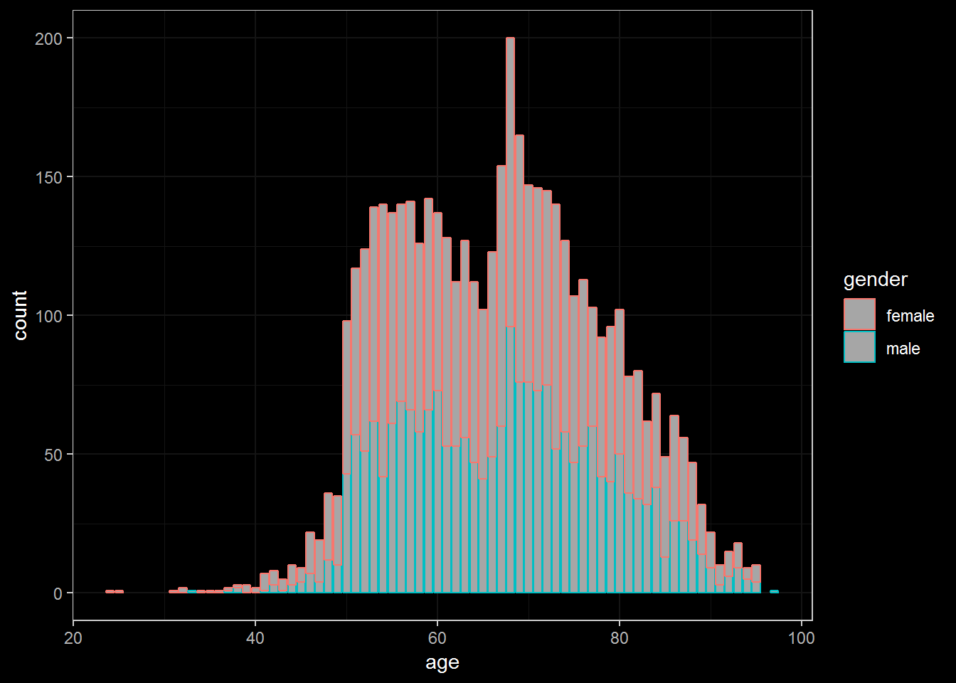

# spike at 68 — what do you think explains this?

The first chunk of the code reduces the nshap dataframe into two variables (age and gender), then converts age into a numeric variable. This reduced dataframe is saved as df_age.

Then, we start the graph with the command ggplot(), set the graph type as a bar graph (again, histogram is the default) with geom_bar. The aes() function here stands for “aesthetics” for the graph, where you set out what R needs to draw. In this case, it draws x-axis with the variable age, and it automatically assigns different colors to different discrete values of gender variable. We give a nice dark theme template look for the graph. Because this is a histogram, we do not need to assign a $y$ variable — it just counts up the number of occurrences for each of the age values.

3.3 Normal bar graph

Instead of the default histogram, let’s try making a normal bar graph.

nshap$maritlst <- factor(nshap$maritlst, levels=c("married",
                                            "living with a partner",
                                            "separated",
                                            "divorced",
                                            "never married",
                                            "widowed"))

marital <- nshap %>% 
    group_by(maritlst, gender) %>% 
    summarise(n = n())

marital %>%
    ggplot() +
    geom_bar(aes(y = n,
                 x = maritlst,
                 colour = gender),
             stat = "identity") +
    ggtitle("Count of respondents vs. marital status by gender") +
    dark_theme_bw()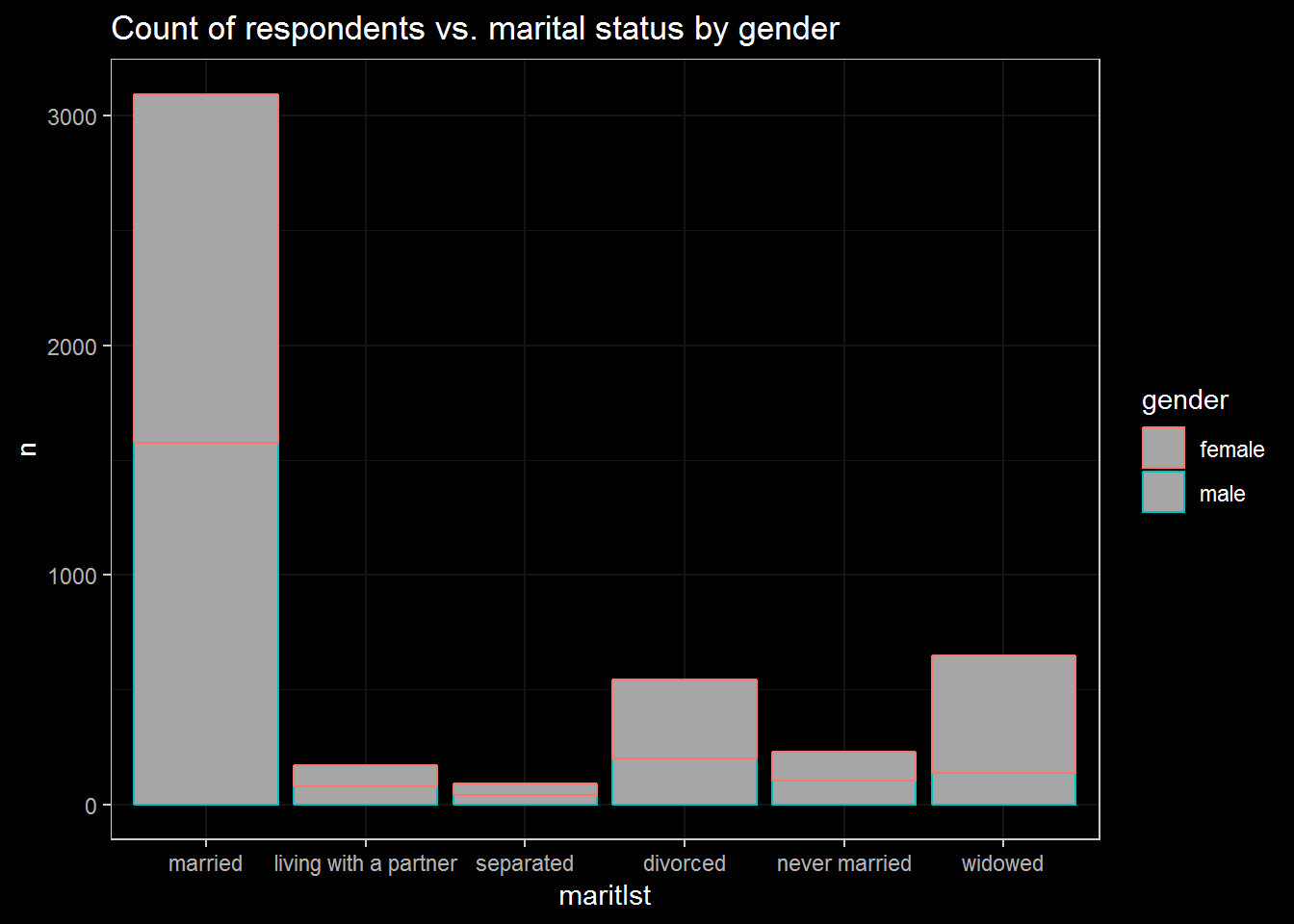

# More widowed females, possibly explained by male deaths from war,
# lower life expectancy for males, etc.

The necessary arguments are y for aes(), stat for geom_bar(). While this is still a histogram because it uses counts (n), this is to demonstrate how to make a normal bar graph. stat = "identity" is what sets it as a normal bar graph and requires you to input the y argument. Then you can put in the title of the graph with ggtitle().

3.4 Switching the axes

Sometimes, the labels might be too long for readability, therefore difficult to fit into the x-axis. You can either choose to rotate the labels so the text becomes vertical, or switch the axes. Below code shows how to switch the axes.

nshap$par_nerve <- factor(nshap$par_nerve, levels=c("often",
                                                    "some of the time",
                                                    "hardly ever or rarely",
                                                    "never",
                                                    "refused",
                                                    "don't know"))

nerve <- nshap %>%
    group_by(par_nerve, gender) %>% 
    summarise(n = n())

#head(nerve)

nerve %>% 
    ggplot() +
    geom_bar(aes(y = n,
                 x = par_nerve,
                 colour = gender),
             stat = "identity") +
    ylab("Count") +
    xlab("How often do you find your partner to be annoying?") +
    coord_flip() +
    dark_theme_bw()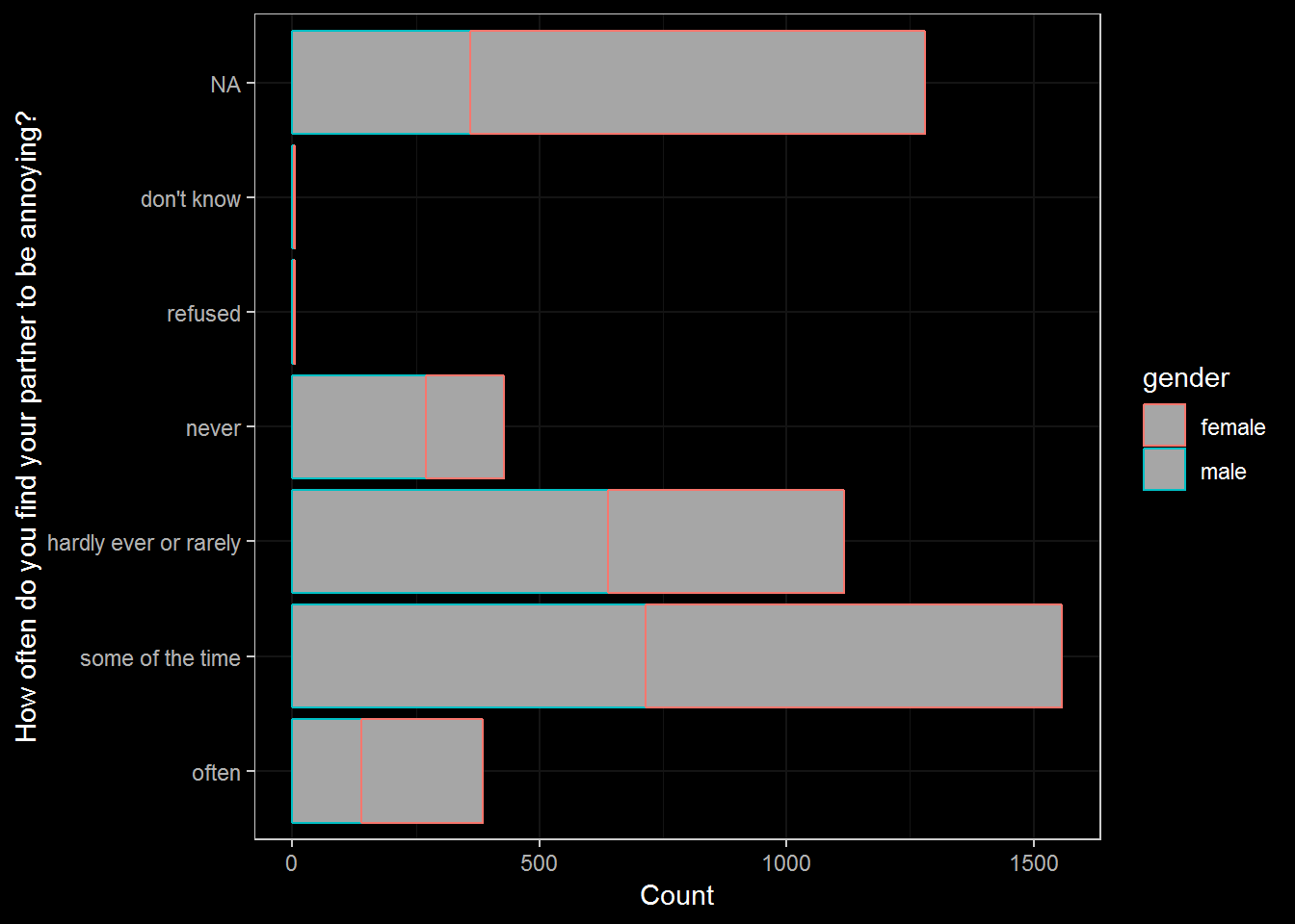

# Looking at raw averages of the respondents, males tend to be annoying
# more frequently, but have to watch out for missing data, indicated by
# "NA" here

coord_flip() flips the $y$ and the $x$ axes, making the graph a horizontal bar graph.

3.5 `geom_smooth()`

A scatter graph is nice when there are only several data points, maybe fewer than 100. However, NSHAP data is rather sizable, which makes geom_smooth() a neat solution that uses LOESS (local estimation scatterplot smoothing) method by default (AKA moving regression similar to moving averages). It also shows 95% confidence interval area, shaded in the graph by default. The CI can be problematic when there are few data points to work off of for some of the local domains, for common example, the extreme income brackets.

hag <- nshap %>% # hearn, age, gender
    select(hearn, age, gender, educ) %>%
    mutate(hearn = as.numeric(hearn),
           age = as.numeric(age))

hag <- na.omit(hag)

hag$educ <- factor(hag$educ, levels=c("bachelors or more",
                                      "voc cert/some college/assoc",
                                      "hs/equiv",
                                      "< hs"))

plotted <- hag %>%
    ggplot() +
    geom_smooth(aes(y = hearn,
               x = age,
               colour = educ)) +
    facet_wrap(~gender) +
    ylab("Household earnings") +
    xlab("Age") +
    ggtitle("Household earnings vs. age") +
    dark_theme_bw(base_size = 11) +
    scale_y_continuous(labels = scales::dollar)

plotted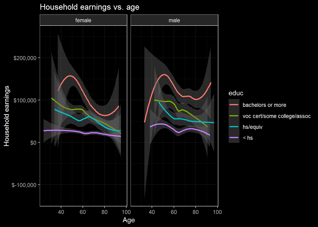

The graph is a bit ugly, but there are several new elements here. Let’s go over them one by one, then address the graph readability later.

First, the graph is saved into the object named plotted.

facet_wrap(~gender): splits the graph into gender‘s (two) discrete values’ graphs.
ylab: y-axis label — similar story applies to xlab and ggtitle.
scale_y_continuous(labels = scales::dollar): R recognizes dollar scale and prepends “$” into the y-axis values.
coord_cartesian(ylim = c(0, 250000)): only shows $y$ coordinates between the set min and max values (but does not remove the values outside of the range from the data; for more, see “clipping” below).

3.5.1 Clipping

knitr::include_graphics("clipping.png")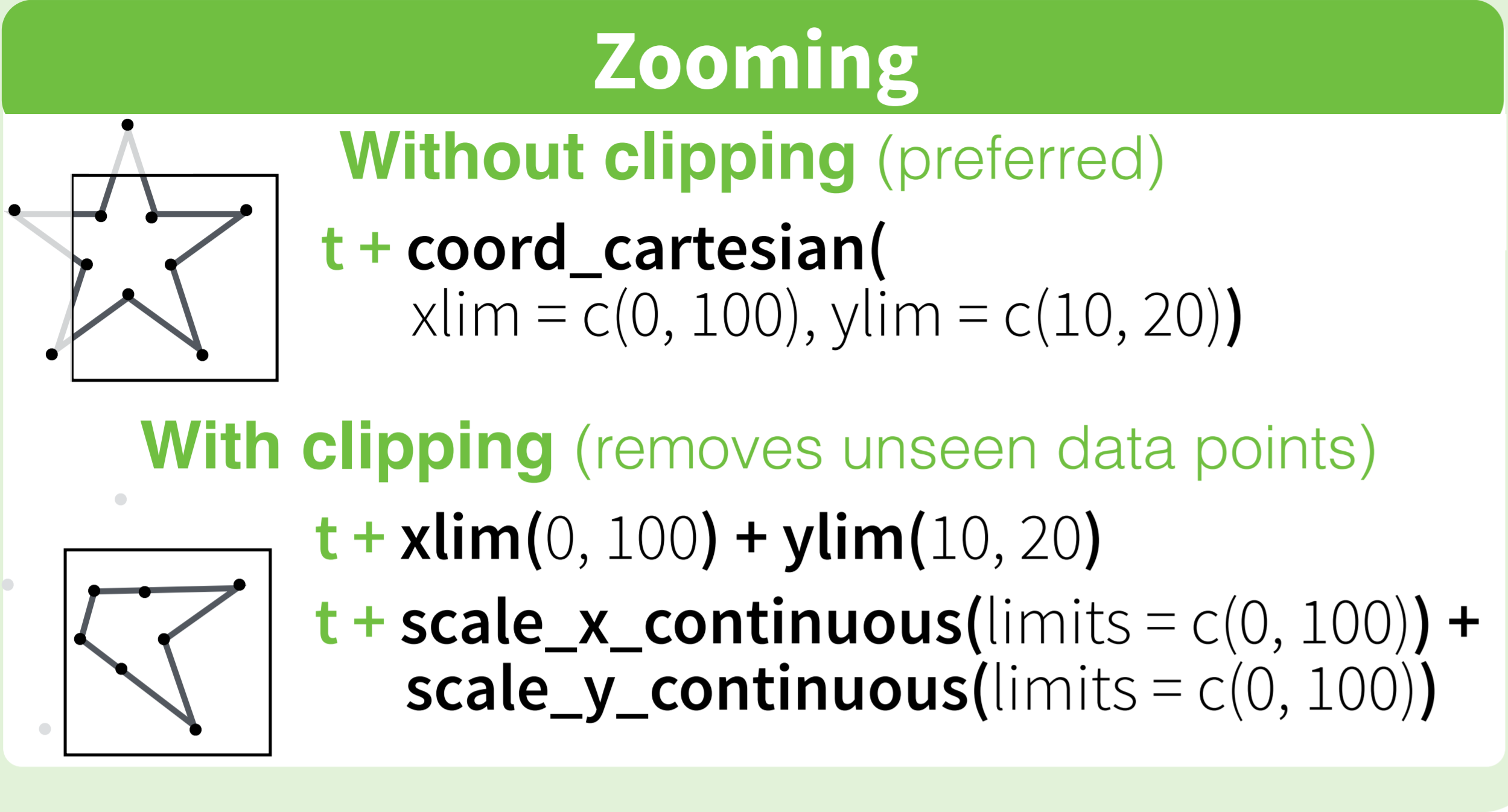

Here, t is the ggplot2 graph object. knitr::include_graphics shows the image file in this tutorial.

3.6 Saving the graph

Conveniently, ggplot2 has its own function to save graphs which makes it simple and convenient. Base R options for saving graphics is not recommended.

ggsave(filename = "hearn_vs_age.png",
       plot = plotted,
       width = 12.8,
       height = 7.2,
       dpi = 150)

knitr::include_graphics("hearn_vs_age.png")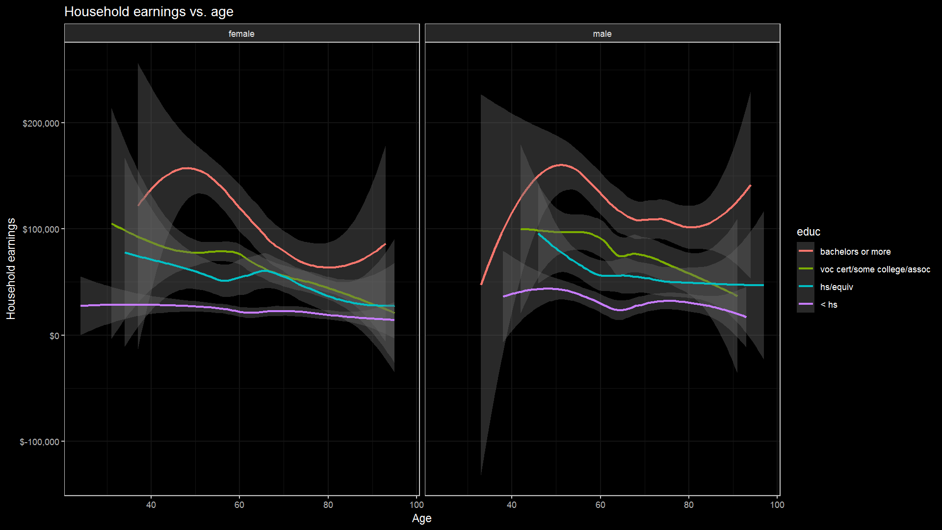

Notice that the graph, fonts, legend, borders, etc. are all rescaled according to the ggsave() arguments and looks much better. You can tweak around with these settings to improve readability as opposed to the previous ugly default graph.

Part 3 Plotting, using ggplot2